The local shape of LLM stable regions

May 18, 2026 · Noah Golmant

This post tries to answer a question about what transformers do at inference: how far can you perturb the residual stream at some position before the predictive distribution changes?

The residual stream is the running per-token vector that gets multiplied by the unembedding $W_U$ to produce next-token logits. (Sometimes called pre-logit activations.) I find this question interesting because it can potentially offer a conceptual insight into the underlying geometry of the distribution and the model’s learning dynamics. It’s also motivated by Janiak et al. 2024, who recently observed “stable regions” in the embedding space (plateaus of output stability along certain interpolation paths, separated by sharp jumps) and asked how big they are and what determines them.

Concretely, let $x \in \mathbb{R}^d$ be the residual stream, and $p = \text{softmax}(W_U x)$ be the predictive distribution. What is the largest $\delta$ along a unit direction $v$ such that $\text{KL}(p_x \| p_{x + \delta v}) < \tau$ for some small threshold $\tau$?

It turns out that in certain interesting cases, there’s a well-defined answer. Define

$$H(x) = W_U^\top (\text{diag}(p) - p p^\top) W_U \;\in\; \mathbb{R}^{d \times d}.$$

Then the predicted boundary distance along $v$ is

$$\delta_{\text{pred}}(v) = \sqrt{\frac{2\tau}{v^\top H(x) v}}.$$

That’s it! $H(x)$ is computable from things already lying around at inference time (the softmax output and the unembedding matrix). And empirically the prediction has two surfaces of usefulness.

Along the highest-curvature direction at small $\tau$, the formula is near-exact: within 1% of the empirical KL boundary on Qwen3-1.7B, and within 8% across three transformer LMs I tested (Qwen, Llama-3.2-1B, Pythia-1B).

For other directions and larger $\tau$, a single isotonic calibration on $\delta_{\text{pred}}$ recovers much of the systematic bias. At $\tau = 1$ nat (a large perturbation magnitude the sampler would notice), the calibrated prediction lands within 50% of the empirical boundary on 54–73% of measurements, depending on architecture.

This post explains where the formula comes from, where it’s accurate, where it needs calibration, and what controls this behavior. And why this is interesting!

Three framings of the same matrix

$H(x)$ can be seen in a few ways.

Second-order Taylor expansion of KL. Treat the predictive distribution as a function of $x$. The KL divergence between $p_x$ and $p_{x+\delta v}$ is zero at $\delta = 0$. Its first derivative is zero (score has mean zero). Its second derivative is exactly $v^\top H v$. Setting $\tfrac{1}{2} \delta^2 v^\top H v = \tau$ and solving gives the prediction above. The formula is a Taylor expansion.

Local curvature of the next-token loss. If you set $L(x) = -\log p(y \mid x)$ for some target token $y$ and ask about the Hessian $\partial^2 L / \partial x \partial x^\top$ at the current residual stream, the answer is exactly $H(x)$. The Hessian doesn’t depend on which $y$ you picked, because softmax is in the exponential family. The per-sample Hessian only depends on $p$, not on the conditioning label. So $H(x)$ describes how sharply the loss bends around $x$ along every direction at once, and our prediction $\sqrt{2\tau / v^\top H v}$ is essentially asking “how far do I walk along $v$ before the loss curves up by $\tau$ nats.”

Fisher information pulled back through the unembedding. The Fisher information of $p = \text{softmax}(z)$ with respect to its natural parameters $z$ is $\text{diag}(p) - p p^\top$. The residual stream parametrizes $z$ via $z = W_U x$, so the Fisher pulled back to $x$-space is $W_U^\top (\text{diag}(p) - p p^\top) W_U$. This is the standard Fisher-information-as-Riemannian-metric construction, restricted to the residual stream.

These are mathematically equivalent for exponential-family losses. The framings are useful because they suggest different intuitions about where the matrix should be useful. The second one, Hessian-of-cross-entropy, is the one that’s most precise about why the prediction works in the operating regime we’ll see below.

Yes-of-course

There’s a reasonable objection at this point: of course a second-order Taylor expansion is accurate for a sufficiently small perturbation. That’s calculus. The interesting parts are empirical:

1. The perturbation magnitudes at which the prediction is useful are not small. For typical KL thresholds (0.1–1.0 nats), the predicted $\delta$ is a non-trivial fraction of $\|x\|$.

2. The prediction is direction-discriminating. Given a position $x$, Fisher correctly identifies which directions move the predictive distribution faster than others under perturbation. The natural test for this is rank correlation between predicted and empirical boundary distances across a sweep of perturbation directions, because we care that the ordering matches even when the absolute magnitudes don’t (the latter is a separate calibration question, addressed below). Per-position Spearman $\rho$ ranges from 0.66 to 0.98 across three architectures and ~50 directions per sweep. The constant baselines (entropy, maximum token probability, trace of $H$) trivially can’t beat zero, because they predict the same boundary distance for every direction.

3. Outside the regime where the prediction is near-exact, the local Fisher quadratic systematically overshoots or undershoots depending on direction class. A single monotone calibration on $\delta_{\text{pred}}$ removes the bias, getting the median calibrated prediction within 50% of empirical out to $\tau = 1$ nat (with a tail though, we’ll see that below).

4. The formula directly addresses the Janiak et al. stable-regions observation from the intro: $H(x)$ is the underlying geometric object, and the closed-form $\delta_{\text{pred}}(v)$ tells you the local direction-specific size of these regions.

Math: the rank-1 regime

Start with the chain-rule derivation. With $z = W_U x$, softmax identities give $\partial p_i / \partial z_j = p_i(\delta_{ij} - p_j)$, so

$$\frac{\partial^2 L}{\partial z_i \partial z_j} = p_i (\delta_{ij} - p_j) = (\text{diag}(p) - p p^\top)_{ij}$$

and since $z = W_U x$ is linear,

$$\frac{\partial^2 L}{\partial x \partial x^\top} = W_U^\top (\text{diag}(p) - p p^\top) W_U = H(x).$$

The matrix $\text{diag}(p) - p p^\top$ is the covariance of the categorical sampling distribution, positive semi-definite with rank $V - 1$. After pullback through $W_U$, the effective rank of $H(x)$ is bounded by the number of tokens with non-negligible probability mass, since rows of $W_U$ at zero-probability tokens contribute nothing.

That last point matters. At many positions during inference, the predictive distribution is dominated by two tokens (call them $i$ and $j$) with $p_i + p_j \approx 1$. In that limit, restrict $\text{diag}(p) - p p^\top$ to the support $\{i, j\}$ and use $p_i(1 - p_i) = p_i p_j$:

$$H(x) \;\approx\; p_i \, p_j \cdot (W_U[i] - W_U[j]) \, (W_U[i] - W_U[j])^\top.$$

This is a rank-1 outer product. Its single nonzero eigenvalue is $p_i p_j \cdot \|W_U[i] - W_U[j]\|^2$ along eigenvector $W_U[i] - W_U[j]$, which is the direction along which an infinitesimal $\delta$ steers the logit difference $z_i - z_j$. The highest-curvature direction of the residual stream, in this limit, is the difference of the two competing tokens’ unembedding rows.

This is the regime where the closed form is most accurate. The Fisher pullback has been reduced to a single nonzero eigenpair, and at small $\tau$ the KL between the original $p$ and a perturbation along that eigenvector is well-described by its second-order expansion (the higher-order terms remain small as long as $\tau$ stays small). Empirically: across three architectures I tested, the top eigenvector of $H_k(x)$ at $k=8$ (which captures essentially all the curvature) is within 8% of closed-form-exact at small $\tau$.

Empirics

I sampled ~4000 positions per architecture (Qwen3-1.7B, Llama-3.2-1B, Pythia-1B), drawn from math (GSM8K), code (codeparrot-clean), dialogue (UltraChat), and wikitext. A position is one tokenized context, with $x$ taken as the post-final-norm residual stream at a target index just before next-token prediction. Sampling was rank-stratified: I bucketed positions by effective Fisher rank quintile and aimed for roughly even coverage, rather than letting the natural distribution oversample the very-confident (rank ≈ 1) end.

For each position I computed $H_k(x)$, a top-$k$ truncation of $H(x)$ that restricts the inner covariance to the top-$k$ tokens by mass before pulling back through the corresponding rows of $W_U$. I used $k=8$; tail tokens contribute negligibly.

I then built a ~50-direction sweep per position: top eigenvectors of $H_k$, structured pairs $W_U[i] - W_U[j]$ for the top-4 tokens, random unit directions, tangent-projected variants, and a negative-control class of directions orthogonal to the top-$k$ active tokens.

For magnitude, define $z = \tfrac{1}{2} \delta_{\text{emp}}^2 \cdot v^\top H v$, the local Fisher quadratic evaluated at the empirical boundary $\delta_{\text{emp}}$ (found by binary search at $\tau \in \{0.01, 0.05, 0.1, 0.5, 1, 2\}$ nats along each direction). If the second-order Taylor were exact, $z$ would equal $\tau$. The rank-1 derivation predicts that the top eigenvector of $H_k$ should be a near-exact direction at small $\tau$. It is:

arch	median $z/\tau$ at $\tau=0.01$ on top-eigvec	95% CI
Qwen3-1.7B	1.002	[0.999, 1.005]
Llama-3.2-1B	1.054	[1.047, 1.062]
Pythia-1B	1.080	[1.072, 1.092]

Qwen is the cleanest, within 1%. The Qwen number is a mean across four independent seeds (per-seed range 0.998–1.004), so the exactness isn’t a single-seed coincidence. The pattern at higher Fisher ranks differs across architectures: on Qwen the curve decays monotonically (rank=7 sits at $z/\tau \approx 0.43$); on Llama and Pythia all seven ranks stay within ~10% of exact. The dominant-direction exactness is universal; the higher-rank shape is model-specific.

Now stratify $z/\tau$ at $\tau = 1$ nat (where you’d actually use the prediction in practice) by direction class:

direction class	Qwen	Llama	Pythia
structured ($W_U[i] - W_U[j]$)	1.05	1.44	1.44
tangent-projected	1.64	1.81	1.74
random	0.23	0.45	0.50
eigvec of $H_k$ (pooled ranks 1–7)	0.12	0.56	0.72

At $\tau = 1$ nat the raw closed form is meaningfully off everywhere except the small-$\tau$ top-eigenvector regime. Structured and tangent directions overshoot ($\delta_{\text{pred}}$ predicts a boundary farther than empirical); random and eigvec undershoot. This is what calibration fixes.

It’s worth noting why the higher eigvecs of $H_k$ (ranks 2–7 pooled) look bad while rank-1 looks great. The top eigvec in the rank-1 regime is essentially $W_U[i] - W_U[j]$, the structured direction, and infinitesimally moving along it only changes $z_i - z_j$, the logit gap between the two competing tokens. KL between two near-binary distributions parameterized by their logit gap stays well-approximated by its second-order expansion as long as the gap stays small. But the rank-2..7 eigvecs by construction excite tokens that weren’t in the top-2 of the original $p$. The moment those tokens pick up appreciable mass, the system stops being binary and the rank-1 simplification no longer holds, so the higher-order terms of the Taylor expansion stop being negligible. So “eigvec, pooled” contains one direction that the closed form describes well and several that it doesn’t, by construction.

A per-class monotone (isotonic) recalibration on $\delta_{\text{pred}}$ fixes most of the bias. Class here means direction class (eigvec, structured, random, tangent), not corpus domain. Fit a single sklearn isotonic regression per class on $(\delta_{\text{pred}}, \delta_{\text{emp}})$ pairs, apply it to held-out positions via 5-fold by-position cross-validation. Pooled across all four classes the calibrator is even simpler (one global isotonic) and gets you most of the way:

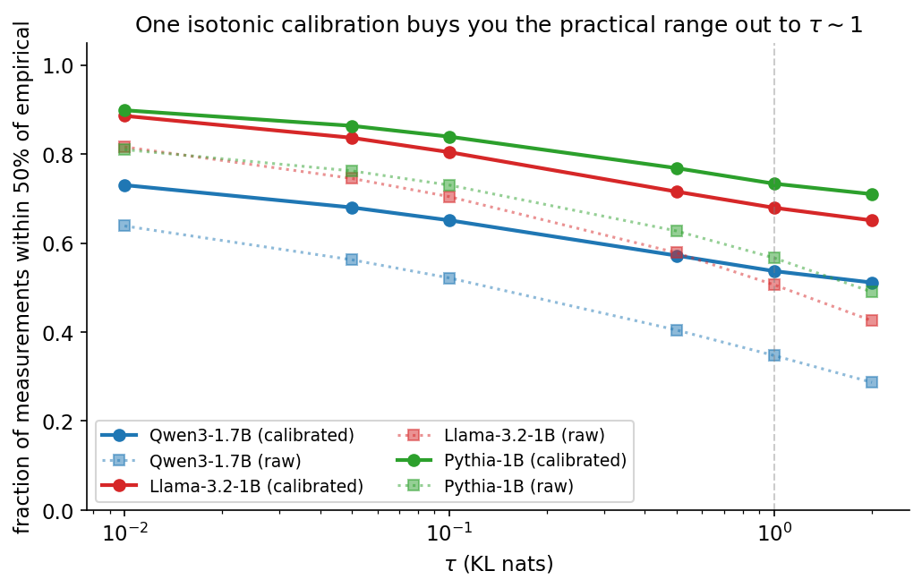
At $\tau = 1$ nat, the pooled isotonic-calibrated $\delta$ lands within 50% of the empirical boundary on 54% (Qwen), 68% (Llama), 73% (Pythia) of measurements; raw uncalibrated, the numbers are 35% / 51% / 57%. Per-class calibration tightens the random class to 76–86% within 50% across the three architectures. Llama and Pythia stay above two-thirds within 50% out to $\tau = 2$. Per-class results spread substantially: at $\tau = 1$ on Qwen, eigvec sits at 32% within-50% while random hits 76%. The pooled headline averages over genuinely different per-class behaviors.

The Fisher-rank story also lets us answer a side question: which property of the position best predicts whether the closed form will work? I pre-registered three candidates (predictive entropy, max top-1 probability, effective Fisher rank), and entropy is the cleanest stratifier across all three architectures. Effective Fisher rank, which I started the study expecting to be the natural axis, is dramatically worse (within-cell variance 30 to 3000 times higher than entropy, depending on architecture). So low-entropy positions sit in the rank-1 regime where the closed form is near-exact along the highest-curvature direction; high-entropy positions spread Fisher mass across several eigenvectors and need the calibration step.

Stable regions, reframed

In this framing, Janiak et al.’s “stable regions” are the geometric image of low-curvature directions in the Fisher pullback metric. A stable region around $x$ extends far along directions where $v^\top H v$ is small (predicted $\delta$ large) and contracts along directions where it’s large. The shape is an ellipsoid in residual-stream space with axes along the eigenvectors of $H_k(x)$ and axis lengths $\sqrt{2\tau / \lambda_i}$. The smallest axis is $W_U[i] - W_U[j]$ scaled by $1/\sqrt{p_i p_j}$, the direction that swaps the model’s top two candidates. The largest axes are directions where Fisher’s predicted curvature is small, and along which the prediction is most prone to overshoot, because rank-1 can collapse and be replaced by new dominant pairs.

Limitations

• Three architectures isn’t many, and Llama and Pythia are single-seed (Qwen is multi-seed, four total).

• KL is the canonical metric. It’s what the closed-form $\delta = \sqrt{2\tau / v^\top H v}$ actually predicts. You could ask the same question with other definitions of “predictive distribution changed” (cosine distance between distributions, argmax flip, etc.), but those don’t have the clean closed-form story.

• The Qwen-specific deep eigvec-rank decline (rank=7 at $z/\tau \approx 0.43$ on Qwen, near-1 on the others) isn’t explained mechanistically. Layer count is a partial correlate (Qwen has 28, the others 16), but Llama and Pythia both have 16 layers and show different per-rank depths, so that alone doesn’t determine it.

Two applications

The more natural fit is mechanistic interpretability. A closed-form local descriptor of “which directions are sensitive at this residual-stream position” could be useful: it lets you ask, for a given internal state, which token-pair competitions are active, how far you’d have to push the residual stream to swap them, and what other geometric properties of $W_U$ correlate with the model’s local sensitivity. That said, I’m not super familiar with the literature in this space.

The more practical-but-shakier direction is speculative decoding. Entropy-based draft-stopping rules like AdaEDL use scalar uncertainty signals to decide when to halt drafting. The closed-form Fisher prediction is directional, not scalar, so it doesn’t drop in directly. The natural scalarization (calibrated $\delta_{\text{pred}}$ along the top eigenvector of $H_k$) is more expensive to compute than entropy and not obviously more informative for acceptance prediction. But maybe there’s something there!

Closing

The math is just a second-order Taylor expansion with a textbook Hessian/Fisher identity, and is most accurate in the regime where the model is essentially solving a binary classification.

What’s surprising is that the prediction is empirically meaningful at non-trivial perturbation magnitudes — perturbations that are appreciable fractions of $\|x\|$ — and that this is a common regime at inference time. And outside this regime, monotone calibration captures much of the systematic bias.

This is a slightly narrower claim than “Fisher pullback explains stable regions”. It’s more like “Fisher pullback predicts stable region boundaries near-exactly along the natural geometric direction, and within a transferable constant elsewhere.” But I think it’s still cool.

Happy to share code and data on request.

Related work worth mentioning: Janiak et al. for the empirical phenomenon this is trying to explain, Mabrok 2026 for an earlier introduction of the same metric in support of static manifold analyses, and Park, Choe, and Veitch 2024 on the geometry of $W_U$ rows in the linear representation hypothesis.